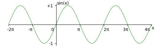
In this post I want to explain a method that gets used a lot in physics to understand both very simple and very complex systems. The goal is to show you how physicists think about these problems, and why this method is so useful, but avoiding doing any of the tedious algebra. I will write down some equations, and I’m going to explain what they mean, but you don’t need to know how to solve them. This post should be understandable without knowing any maths other than the shape of a sine curve:

If you’ve heard the any of these terms:

• normal modes
• small perturbations
• linear modes
• natural frequencies
• resonance

then this post should explain what these mean. You can ignore the footnotes.

If you want to learn how to use this method, then read the footnotes. I’ll give a little more of the maths there, and tell you what to look up to actually use this technique.

Small oscillations

We’re going to understand the physics of small oscillations of systems. The word “system” might sound ambiguous and wishy-washy, but that’s deliberate: what we’re going to talk about occurs in systems as simple as a pendulum, up to objects as complex as an aircraft. It’s also applicable to guitar strings, drum-skins, water waves, and even stars. (I wrote this post because I began writing a post to explain my PhD thesis, which was partially about using this method in the context of stars. Partway through I realized that I was writing a long explanation about linear modes, and decided to break it out into this post.) It even forms the basis of quantum electrodynamics, the theory of how light interacts with electrons, although in that case there are other complications.

Why small oscillations? The answer is partly “because those are the ones where we can solve the equations”. Partly it is because, for most systems, oscillations start small. This method lets us estimate if they will stay small. If the oscillations are vibrations in the wing spar of an aircraft, we want them to stay small!

Why not run a computer simulation instead, and get exact answers? Sometimes this is the best solution. It may well give us the most accurate numbers. But it is much harder to extract understanding from a simulation. Designing a system (a bridge, an aeroplane, a drum) would consist of guessing, running a simulation, and repeating the process with a slightly different guess, ad nauseam. Even if the simulation is quick to run, this process will be extremely slow if there are lots of design parameters that we can change. A much better process is to design our system based on how its small oscillations behave, and then run a simulation that correctly models larger oscillations and check that everything is still acceptable. There is also the issue of how confident we are that our computer simulation is correctly implemented. One test of this is “does it behave the way it should for small oscillations?”.

Pendulums

A pendulum is about the simplest system you can imagine. You can build one by tying a nut to the end of a length of string.

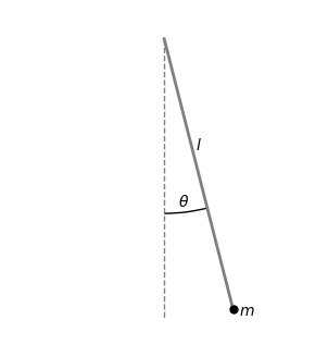
We’ll call the length of the string \(l\), and the mass of the bob \(m\). So long as the string stays taut, we can describe the state of the pendulum at any moment of time by its angle from the vertical, \(\theta\). This is an example of what we call a degree of freedom of the system. The pendulum is very simple because it has only one degree of freedom.

We can work out the equation of motion for this system. It turn out to depend on \(l\), and the local gravitational acceleration, \(g\), (\(g = 9.81 \mathrm{m}/\mathrm{s}^2\) on Earth), but not on the mass of the pendulum: \[ \frac{\mathrm{d}^2 \theta}{\mathrm{d} t^2} = - \frac{g}{l} \sin \theta \] Don’t worry if you don’t know any calculus. The thing on the left hand side, \(\mathrm{d}^2 \theta / \mathrm{d} t^2\), is the acceleration of \(\theta\). It’s not its speed. The equation of motion doesn’t directly determine the speed. It’s how fast the speed is changing.

Let’s plot the right hand side:

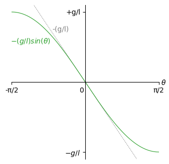
I’ve only plotted this up to \(90^{\circ}\) in either direction, since beyond that the string isn’t going to remain taut.

For positive \(\theta\), this is negative. It’s going to accelerate the pendulum back towards \(\theta = 0\). You know this from experience, it isn’t surprising. Unless you push the pendulum bob really hard from the bottom, it will swing back. We call this the restoring force, since it tries to restore the pendulum to one particular point.

But look at the gray dashed line. You can see that a straight line is a really good approximation to the restoring force as long as the angle is small. In fact, the difference is less than \(1\%\) as long as \(\theta\) is less than \(14^{\circ}\). If we only want to know how the pendulum behaves for small angles, we could make this approximation, and use the simpler equation of motion \[ \frac{\mathrm{d}^2 \theta}{\mathrm{d} t^2} = - \frac{g}{l} \theta \]

We say that this equation is “linear in \(\theta\)”. This means that if we replace \(\theta\) by any multiple of \(\theta\), the equation is still true. This is why this method is often referred to as finding the linear modes of the system.

There are things where the restoring force cannot be approximated by a straight line, even very close to the point where the system is at rest.¹ But for most real-world systems this is a good approximation in some circumstances, and that makes it a useful approximation.

Why is approximating \(\sin \theta\) as just \(\theta\) useful? Because we can now solve the equation of motion, and find how \(\theta\) changes over time:²

\[ \theta (t) = A \sin \bigg(\sqrt{(g/l)} ~ t + \varphi_0\bigg) \]

Here’s what that motion looks like:

Two new variables have appeared: \(A\) and \(\varphi_0\). We call \(A\) the amplitude and \(\varphi_0\) the initial phase. Any values of these give a solution to the equation of motion. In other words, the equation of motion does not tell us what \(A\) or \(\varphi_0\) should be. But that makes sense: the equation of motion doesn’t tell us the starting position of the pendulum, or how fast it’s moving.

Here are three solutions to the equation of motion with different amplitudes and phases:

Whatever \(A\) or \(\varphi_0\) are, the pendulum will do one cycle in the same time period: \(2 \pi \sqrt{\frac{l}{g}}\). If you make the string 99.4 cm long, you’ll get a period of 2 seconds, just like the animations above. It doesn’t matter what the mass of the bob is (so long as it’s much heavier than the string), and it does not depend on what the amplitude of the oscillations are. That second part is extremely useful - it’s why pendulums are a good way for a clock to keep time.

The combination \(\sqrt{(g/l)}\) is called the angular frequency, and is usually denoted \(\omega\). It has units of \(\mathrm{rad} / s\), read as “radians per second”. It’s more common to talk about frequency in Hertz (Hz), which is usually denoted \(f\) and is the number of complete cycles in one second. The time to do a complete cycle is denote by \(T\). They’re related by \[ f = \frac{\omega}{2 \pi} = \frac{1}{T} \] People like to think in terms of \(f\), but formula are usually shorter in terms of \(\omega\).

More degrees of freedom

The pendulum has a single degree of freedom. Can we apply this method to a system with two degrees of freedom? Well one really obvious example is a pair of pendulums. Their linearized equations of motion are \[ \begin{align} \frac{\mathrm{d}^2 \theta_1}{\mathrm{d} t^2} &= - \frac{g}{l_1} \theta_1 \\ \frac{\mathrm{d}^2 \theta_2}{\mathrm{d} t^2} &= - \frac{g}{l_2} \theta_2 \end{align} \] with solution \[ \begin{align} \theta_1 (t) &= A_1 \sin \bigg(\sqrt{(g/l_1)} ~ t + \varphi_1\bigg) \\ \theta_2 (t) &= A_2 \sin \bigg(\sqrt{(g/l_2)} ~ t + \varphi_2\bigg) \end{align} \]

Here they are with different phases and amplitudes. I’ve made the pendulums different lengths so that they have different frequencies:

I think you will agree that this isn’t really adding anything new. It’s just two copies of the pendulum solution. It feels like cheating to claim this is a system with two degrees of freedom.

A much more interesting system is a double pendulum:

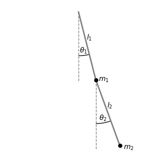
I’m going to assume our double pendulum has bobs with masses in the ratio \(m_1 / m_2 = 16/9\), simply because this makes some numbers come out nicer. I’m also going to assume that the strings have the same length: \(l_1 = l_2 = l\).

This really is a system with two degrees of freedom, \(\theta_1\) and \(\theta_2\). The equations of motion are quite complicated,³ but just like the regular pendulum we can construct linearized versions of them: \[ \frac{\mathrm{d}^2 \theta_1}{\mathrm{d} t^2} + \frac{9}{25} \frac{\mathrm{d}^2 \theta_2}{\mathrm{d} t^2} + \frac{g}{l} \theta_1 = 0 \\ \frac{\mathrm{d}^2 \theta_2}{\mathrm{d} t^2} + \frac{\mathrm{d}^2 \theta_1}{\mathrm{d} t^2} + \frac{g}{l} \theta_2 = 0 \]

First, lets just look at what a solution looks like:

At first glance this does not look very understandable. Neither \(\theta_1(t)\) or \(\theta_2(t)\) are nice simple sine curves. There isn’t a simple relationship between them either, like one being the negative of the other. But there’s clearly some kind of order. The whole thing is at least periodic, repeating the same pattern every 2 seconds (this is actually why I chose that relationship between the two masses - it makes this clearer).

I wanted you to see this motion first because once we see the solution to the double pendulum’s linearized equations of motion, it starts to reveal what’s actually going on: \[ \begin{align} \theta_1(t) &= 3 A_1 \sin \bigg( \sqrt{(5g/2l)} ~ t + \varphi_1 \bigg) + 3 A_2 \sin \bigg( \sqrt{(5g/8l)} ~ t + \varphi_2 \bigg) \\ \theta_2(t) &= -5 A_1 \sin \bigg( \sqrt{(5g/2l)} ~ t + \varphi_1 \bigg) + 5 A_2 \sin \bigg( \sqrt{(5g/8l)} ~ t + \varphi_2 \bigg) \end{align} \]

We now have four variables that aren’t set by the equations of motion (\(A_1\), \(A_2\), \(\varphi_1\), \(\varphi_2\)), but that makes sense: we have to also specify the initial positions and velocities of two things (the two pendulum bobs) to know what’s going to happen. We saw exactly the same thing with the two side-by-side pendulums above.

The solutions are still composed of sine functions, with two different frequencies (\(\sqrt{\frac{5g}{2l}}\) and \(\sqrt{\frac{5g}{8l}}\)), but now both frequencies appear in the solution for \(\theta_1(t)\), and they both appear in \(\theta_2(t)\) too. We can see what’s going on much more clearly if we set one of \(A_1\) or \(A_2\) to zero:

In both these motions, everything is a sine curve. We’d call these two forms of motion different modes of the system. There’s a slow mode, with a period of two seconds, where the two bobs move in the same direction. And there’s a fast mode, with a period of one second, where the bobs move in opposite directions from each other.

Now that we have two degree of freedom, telling you the two frequencies does not tell you everything about the system: you also need to know the shape of the motion. You need to know that for the fast mode, \(\theta_2(t) = -\frac{5}{3} \theta_1(t)\), and that for the slow mode, \(\theta_2(t) = + \frac{5}{3} \theta_1(t)\).

I’ve described these two modes by giving you the general solution to the equations of motion, and then pointing out that it’s composed of motion with only two frequencies. In practice, we solve the problem by going in the other direction. We know that equations of motion of this kind, however many degrees of freedom it has, will have solutions that are composed of sine functions.⁴ If the motion is a single mode with angular frequency \(\omega\), then we can replace \(\mathrm{d}^2 / \mathrm{d} t^2\) with \(-\omega^2\). We do this to each equation of motion, do some algebra, and get an equation for \(\omega\). This equation usually has multiple solutions - the same number of solutions as the number of degrees of freedom. Now that we have the frequencies of the modes, we pick one. We put the frequency into the equations of motion, and we find a ratio between the degrees of freedom for that mode. For example, in the double pendulum we found that for \(\omega = \sqrt{\frac{5g}{2l}}\), we need \(\theta_2 = -\frac{5}{3} \theta_1\), and that for \(\omega = \sqrt{\frac{5g}{8l}}\) we need \(\theta_2 = +\frac{5}{3}\theta_1\).

Infinitely many degrees of freedom

In the real world we often want to understand continuous systems that have an enitre dimension’s-worth of degrees of freedom. Imagine a string, like a guitar string. It runs along the \(x\)-axis, but gets pulled away by a distance \(y\) (except at the ends, \(x=0\) and \(x=l\) where it’s pinned in place):

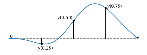
To really describe the string at an instant in time, I need to give you the displacement, \(y\) at every point. If I just gave you, say, the three points shown, then there’s lots of ways you could join the dots to produce different shapes for the rest of the string. I really need to give you a whole function, \(y(x)\), to describe the shape. And then my equation of motion needs to tell me how this function changes over time, and I need to somehow solve that. This turns out to be perfectly doable.

First, let’s write down the equation of motion for our string: \[ \frac{\partial^2 y(x, t)}{\partial t^2} = c^2 \frac{\partial^2 y(x, t)}{\partial x^2} \] We also know that \(y(0, t) = 0\) and \(y(l, t) = 0\), because our string is fixed at the ends.

Some new symbols have appeared. I promised I’d explain what terms in equations mean for anyone who is unfamiliar with calculus, and I will. Because \(y(x, t)\) is a function of two variables, there are two things we can differentiate (find rates of change) with respect to: \(x\) and \(t\). All the \(\partial\) sign means is “find the rate of change with respect to one variable, keeping the other fixed”. So \(\partial^2 y(x, t) / \partial t^2\) is the rate of acceleration at one fixed \(x\) point on the curve - it doesn’t care what \(y\) is doing at any other value of \(x\). And \(\partial^2 y(x, t) / \partial x^2\) is how curved \(y(x, t)\) is in the \(x\) direction - but only at this moment in time, it doesn’t care about any times earlier or later that this \(t\). Finally, \(c\) is called the wave speed, and it’s just a constant.

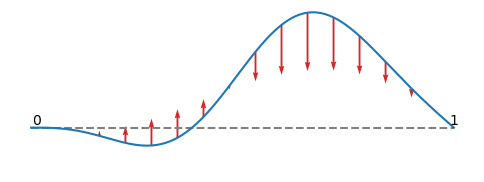
I’ve plotted as arrows above the direction the curvature pulls the string in. You should notice something here: it doesn’t matter how far from the dashed line the string is, or what its gradient is. See that straight section in the middle, around \(x=0.5\), that is displaced upwards? It’s displaced a long way, but the string is quite straight there. There’s no curvature, so it isn’t being accelerated right now.

Remember in the previous section I told you that we usually start by substituting in the assumption that our solution looks like a sine function? Well here we can try that with just the time-dependence. We can try \[ y(x, t) = f(x) \sin (\omega t + \varphi) \] Then our equation of motion becomes (after cancelling \(\sin(\omega t + \varphi)\) from both sides): \[ -\omega^2 f(x) = c^2 \frac{\mathrm{d}^2 f(x)}{\mathrm{d}x^2} \] It doesn’t look like anything about this constrains what \(\omega\) can be, but the equation should look familiar. It’s the same as the linearized equation for the simple pendulum, except with \(x\) instead of \(t\), and \(\omega^2 / c^2\) instead of \(g/l\). Which means we know how to solve this, so we get \[ y(x, t) = A \sin((\omega / c) x + \phi) \sin(\omega t + \varphi) \]

Now we can put some constraints on \(\omega\)! Remember that the string is fixed so that \(y(0, t) = y(l, t) = 0\). Picking \(\phi = 0\) will ensure that \(y(0, t) = 0\).

I did say that I’d expect you to know a little about sine curves. Remember that \(\sin(\theta) = 0\) if \(\theta = n \pi\) for some integer \(n\). So if \((\omega / c) l = n \pi\), our boundary conditions will both be satisfied.

In other words, we’ve found that the allowed frequencies are \[ \omega_n = \frac{n \pi c}{l} \] and that the corresponding shape of the modes are \[ f_n(x) = \sin\bigg(n\pi \frac{x}{l}\bigg) \] We can throw away negative \(n\) (they just change the sign of the amplitude, they’re a repitition of the positive \(n\) modes) and write the general solution as \[ \begin{align} y(x, t) & = A_1 \sin\bigg( \pi \frac{x}{l} \bigg) \sin\bigg( \pi \frac{c t}{l} + \varphi_1 \bigg) \\ & + A_2 \sin\bigg( 2\pi \frac{x}{l} \bigg) \sin\bigg( 2\pi \frac{c t}{l} + \varphi_2 \bigg) \\ & + A_3 \sin\bigg( 3\pi \frac{x}{l} \bigg) \sin\bigg( 3\pi \frac{c t}{l} + \varphi_3 \bigg) \\ & + A_4 \sin\bigg( 4\pi \frac{x}{l} \bigg) \sin\bigg( 4\pi \frac{c t}{l} + \varphi_4 \bigg) \\ & + \dots \end{align} \] We do have an infinite number of amplitudes (\(A_1\), \(A_2\), …) and phases (\(\varphi_1\), \(\varphi_2\), …) to specify, but in practice we can usually ignore these beyond some point.⁵

I don’t think this big sum of sines of space multiplied by sines of time is easy to visualize if you’re seeing it for the first time. I’m hoping the animation below makes it a little clearer. On each row I’ve plotted one of the modes on the left (the blue curve). On the right (the yellow curve) I’ve plotted the sum up to and including that mode. I’ve chosen the wave speed (\(c\)) so that the slowest mode takes 4 seconds to cycle.

You can see that as more modes are added the motion gets more complex. One thing that’s important to note is that it’s not just the amplitude, that \(A_1\), \(A_2\), …, the how much of each mode, that matters. The relative phases, \(\varphi_1\), \(\varphi_2\), …, can strongly affect what the motion looks like too. Here’s the same three modes, but with the second mode changed by \(180^{\circ}\):

You can make almost⁶ any shape you want from summing up sine waves of higher and higher frequencies. This avoids you having to re-solve the equation of motion for different configurations of the string: you find the amplitudes (\(A_1\), \(A_2\), …) and phases (\(\varphi_1\), \(\varphi_2\), …) that describe the initial state of the system. You know how each of those linear modes change over time, because you know their frequencies. To find the state of the system at a later time, you sum these back up.

You can get some remarkably odd things out of this. Here’s an example of a string where we set its initial state to be a triangular displacement.

You can show that this is how the wave equation should behave, with the solution “bouncing” back and forward between the ends of the string. But that’s not how this animation is produced. Instead I’ve split the string up into the individual modes. All you’re seeing in that video is a sum of sine waves oscillating at different frequencies.

What does this get used for?

The real result here is this: If you hit (or push, shake, vibrate) something, so that this displacement is small, it has a set of frequencies it will vibrate at. This is really useful.

If you’re building a bridge, you want all of the vibration frequencies to be a long way from what traffic or weather will produce.⁷ You also want to avoid systems have modes with frequencies that will harm people. In the 1960s a test pilot flying an experimental aircraft, the TSR-2, found himself briefly losing his vision at certain throttle settings. This turned out to be due to part of the aircraft vibrating at the same frequency as the one of the linear vibration modes of the pilot’s eyeball in its socket.

My favourite use of this is in 3D printers. 3D printers are becoming very cheap, and are often shipped as a kit. This limits how rigid they can be. On top of that, they have a few parts that move and change direction very rapidly. Sometimes the frequency of a moving part matches a frequency of the frame, and you get ringing, which shows up as unwanted waves on the surface of the printed object. At least one piece of control software (Klipper) has the option to measure the frequency of the modes of the printer, and then avoids moving any parts at these frequencies.

I originally started writing this because I wanted to describe my PhD reseach in simpler terms, and part of that was about linear modes of stars and planets. In that case the complexity mainly lies in finding the spatial form that the modes can take (which was mostly done in 1889, but in a somewhat hard to understand form), and then understanding how the different modes lose energy, and how strongly they get forced in different situations.

Going further

If you’ve read this and you’re interested in understanding more about this, there’s several places to start.

Knowing how to solve a second order ODE of the form \[ \frac{\mathrm{d}^2 f(x)}{\mathrm{d} x^2} = - \omega^2 f(x) \] in terms of exponentials (\(f(x) = e^{-i \omega t}\)) isn’t strictly essential, but it does make the notation easier and it is the language that a lot of textbooks and lecture notes use.

For higher dimensional systems (e.g. the double pendulum) it helps to understand some linear algebra, in particular Gaussian elimination.

For continuous systems (vibrating strings, drums, waves on the surface of water), you’ll need to understand a little about solving partial differential equations. This is a huge topic, but specifically what you want to look into is the technique of separable partial differential equations. This is essentially what we did when solving the wave equation, by looking for solutions where both sides were separately equal to the same constant: \[ \frac{\partial^2 y{x, t}}{\partial t^2} = -\omega^2 = c^2 \frac{\partial^2 y{x, t}}{\partial x^2} \] and then asking what values of \(\omega\) allow this.